Skip to content
  1. Projects

Unified CNN and GNN model

A vision and movement network in which place, grid and object cells emerged, built end to end and served as a public API.

Unified CNN and GNN model
  • TensorFlow
  • CNN
  • GNN
  • Unity3D
  • EWC
  • FastAPI
  • Streamlit
1M+
trajectory points across all sessions
7
training configs, one network
320
units sorted by rules in code

I designed the Unity simulator, the data pipeline, the model, the code that evaluates it, and the API that serves it. Seven types of hippocampal cells emerged in the network, from nothing more than what an agent sees and how it moves.

What I owned, as first author

  1. ScopeThe question, and which experiments would answer it
  2. Simulator and dataThe Unity room, the paths, the views, the dataset
  3. ModelArchitecture, graph rule, loss switches, EWC
  4. EvaluationClassifier code for all seven cell types
  5. ShippingAPI, interface, hosting, then a review and fixes
  • Top: the 32 × 32 view
  • The agent and its trail
  • Where one unit fires

Research

The problem

The brain has cells for space (place, grid, border) and cells for objects (object sensitive, object, object vector, object trace). Models usually explain one family at a time, and one well known model, the Tolman Eichenbaum Machine, needs a map of the world given to it. Can one network that only sees and moves give rise to both families, with no map at all? And what decides which ones appear?

Five columns. Each shows a 32 by 32 pixel view from the agent and, below it, the room from above with the path. Coloured walls with no object; a cube added; the cube moved; black walls where the view is all black; a circular room.
Figure 1. The sessions, with a real view from each. The object comes, moves and goes; black walls and a round room test what holds.

System design

How it works

The system, end to end Five stages. Simulate: a Unity3D room with a point agent gives exact labels. Data: views shrunk to 32 by 32 and path integration signals, over one million points, hosted as a Hugging Face dataset. Train: one network with vision and movement as graph nodes and three loss switches, giving seven configs, retrained session after session with elastic weight consolidation. Evaluate: a firing map per unit tested against written rules, 320 units sorted into seven types. Serve: weights from the dataset, a FastAPI model server and a Streamlit interface, accepting numpy archives only. 1 · SIMULATE Unity3D room Smooth random paths for a point agent 120° view, rendered at 1171 × 430 Sessions as settings: object, walls, shape Exact labels for every view 2 · DATA Views and paths Views shrunk to 32 × 32 100 path integration signals for movement Hosted as a Hugging Face dataset 1M+ points across sessions 3 · TRAIN One network Vision and movement as graph nodes 3 loss switches: position, heading, reward Sessions in order, memory kept by EWC 7 configs same data and network 4 · EVALUATE Rules in code A firing map for every hidden unit One written test per cell type Thresholds from the published studies 320 units sorted into 7 types 5 · SERVE Two Spaces Weights read from the dataset at start A FastAPI server Streamlit interface Sample in one click .npz only nothing unpickled
The system, end to end Five stages. Simulate: a Unity3D room with a point agent gives exact labels. Data: views shrunk to 32 by 32 and path integration signals, over one million points, hosted as a Hugging Face dataset. Train: one network with vision and movement as graph nodes and three loss switches, giving seven configs, retrained session after session with elastic weight consolidation. Evaluate: a firing map per unit tested against written rules, 320 units sorted into seven types. Serve: weights from the dataset, a FastAPI model server and a Streamlit interface, accepting numpy archives only. 1 · SIMULATE Unity3D room Exact position, heading, reward Point agent on smooth random paths 120° view, rendered at 1171 × 430 Sessions as settings: object, walls, shape 2 · DATA Views and paths 1M+ points across sessions Views shrunk to 32 × 32 Movement as 100 path integration signals Hosted as a Hugging Face dataset 3 · TRAIN One network 7 configs same data, same network Vision and movement as graph nodes 3 loss switches: position, heading, reward Sessions in order, memory kept by EWC 4 · EVALUATE Rules in code 320 units sorted into 7 types A firing map for every hidden unit One written test per cell type Thresholds from the experimental literature 5 · SERVE Two Spaces .npz only nothing unpickled Weights read from the dataset at start FastAPI model server Streamlit interface Sample in one click
Figure 2. Five stages, each one changeable without touching the others.

Exact labels from Unity. I built the room in Unity3D, so every view comes with its exact position, heading and reward.

Two senses, one graph. Vision plays the lateral entorhinal cortex, movement the medial one. A graph layer joins them, with no map given in advance.

Read the hidden layers. After training, each of the 320 hidden units gets a firing map and is tested against the rule for each cell type.

The unified model: two senses, one graph layer, three outputs Two inputs: a 32 by 32 colour view from the agent and 100 path integration signals. Vision goes through one convolution layer with 4 filters and a max pool into 32 LEC units. Path integration goes into 32 MEC units. A graph layer treats LEC and MEC as two nodes of 32 features and mixes them. Three dense layers of 64 units follow. The network predicts position as 22 values, heading as 11 and reward as 1, and each output can be switched on or off in training. The 320 hidden units are read as neurons; the network has 21,362 weights. 1 · WHAT IT SEES The agent’s view, shrunk 32 × 32 × 3 colour 2 · HOW IT MOVED 100 direction waves sin(2π · z·uᵢ) 3 · VISION (LEC) One convolution, 4 filters, max pool 5×5 conv · 32 units 4 · PATH (MEC) One dense layer on the waves 100 in · 32 units 5 · GRAPH LAYER Each sense is a node. They share what they know. LEC MEC Own features plus the mean of both nodes 2 nodes × 32 units 6 · THREE LAYERS Fully connected, like the CA regions D1 D2 D3 64 units each 7 · THREE OUTPUTS Each one can be switched off in training Position11 x + 11 y Heading11 values Reward1 value Shown: config 101 7 configs in all
The unified model: two senses, one graph layer, three outputs Two inputs: a 32 by 32 colour view from the agent and 100 path integration signals. Vision goes through one convolution layer with 4 filters and a max pool into 32 LEC units. Path integration goes into 32 MEC units. A graph layer treats LEC and MEC as two nodes of 32 features and mixes them. Three dense layers of 64 units follow. The network predicts position as 22 values, heading as 11 and reward as 1, and each output can be switched on or off in training. The 320 hidden units are read as neurons; the network has 21,362 weights. 1 · WHAT IT SEES The agent’s view, shrunk 32 × 32 × 3 colour 2 · HOW IT MOVED 100 direction waves sin(2π · z·uᵢ) 3 · VISION (LEC) One convolution, 4 filters, max pool 5×5 conv · 32 units 4 · PATH (MEC) One dense layer on the waves 100 in · 32 units 5 · GRAPH LAYER Each sense is a node. They share what they know. Own features plus the mean of both nodes LEC MEC 2 nodes × 32 units 6 · THREE LAYERS Fully connected, like the CA regions 64 units each D1 D2 D3 7 · THREE OUTPUTS Each one can be switched off in training Position 11 x + 11 y Heading 11 values Reward 1 value Shown: config 101 7 configs in all
Figure 3. Two senses, one graph layer, three outputs that can each be switched off in training. The teal layers hold the 320 units read as neurons.

Judgement

The decisions

What changed between the 2022 notebooks and the final model, and the thinking behind each.

DecisionThinkingEvidence
Drop recurrenceAveraged over time, movement depends on place alone, so memory only slowed training.140 s an epoch, one sample at a time, before
Keep it smallEvery unit had to be readable as a neuron. A bigger network would fit better and explain less.320 units, all tested
Each sense is a nodeKeeping vision and movement apart shows which sense each cell needs.Borders on vision, grids on movement
Population codesPosition and heading spread over many units, the way the brain codes them, not raw numbers.
The objective is the experimentOne network, three loss switches. Any change in the cells comes from what it predicts.Reward alone gave the most object cells
Rules in codeA written test per cell type, with thresholds from the literature, so anyone can rerun the count.
Protect memoryNew object positions erased the memory of old ones in the dark. EWC protects the weights that held it.21 memory cells against 51; EWC raised it

Research

What emerged

Same data, same network. Only the training switches change, and they decide which cells appear.

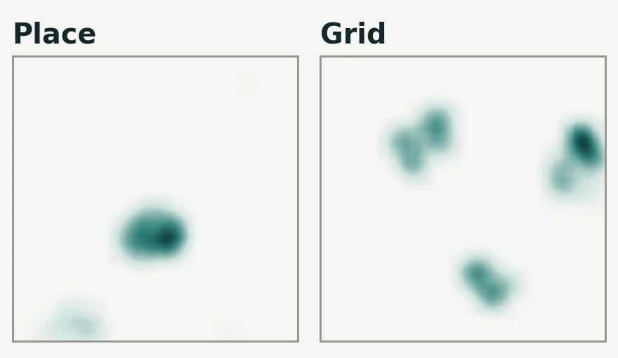
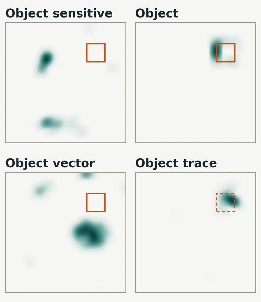
Seven small firing maps in a row, one per cell type: place, grid, border, object sensitive, object, object vector and object trace. Object maps outline the cube in rust.
  • Position
  • Heading
  • Reward
  • Position
  • Heading
  • Reward
  • Position
  • Heading
  • Reward
  • Position
  • Heading
  • Reward
Firing maps of a place cell and a grid cell.
  • Place: I am here
  • Grid: A map grid laid over the room
  • Position
  • Heading
  • Reward
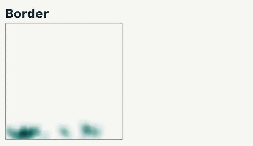
Firing map of a border cell, along one wall.
  • Border: A wall is close
  • Position
  • Heading
  • Reward
Firing maps of object sensitive, object, object vector and object trace cells, with the object outlined in rust.
  • Object sensitive: Something new is in the room
  • Object: Something is here
  • Object vector: It is over there, at this distance
  • Object trace: Something was here
Figure 4. One example of each type. Under each group, the training switches that produced it; rust means on. Rust squares mark the object, dashed where it used to be.
  • PlaceI am here
  • GridA map grid laid over the room
  • BorderA wall is close
  • Object sensitiveSomething new is in the room
  • ObjectSomething is here
  • Object vectorIt is over there, at this distance
  • Object traceSomething was here

Research

A memory of the object

Three firing maps of one cell. Before the object, it fires faintly elsewhere. With the object in the room, still nothing at the object. After the object is learned and removed, it fires strongly where the object used to be.
  • The object
  • Where it used to be
Figure 5. Once the object is gone, this cell fires where it used to be.
  • 105 of 131place cells kept their field in the dark
  • 36 of 72object cells moved with the object
  • 51cells kept a memory of the object

Limits

  • Movement is idealisedPath integration is a function of position, not integrated velocity.
  • Overlapping labelsOne unit can pass two rules, for example place and object trace.
  • Grids bendGrid cells lost their pattern when the room changed: 24 of 50 kept it in a circle.
  • Borders need sightIn the dark only 4 units stayed border cells. Touch as a third node would help.

Next: real limb movement as the input to path integration, and an agent that navigates.

Product

Shipping, then reviewing my own system

I split the research code into two Docker Spaces, then reviewed the live API as if someone else had built it.

How the live demo is built A visitor's browser opens a Streamlit Space, which holds no model and only calls the API. A separate FastAPI Space serves the model with three endpoints: sample, inference and layers. It loads the weights once at startup from a Hugging Face dataset holding the weights and data for all seven configs. Uploads are numpy archives only. Visitor Any browser SPACE 1 · DOCKER INTERFACE Streamlit port 7860 Run the sample in one click No model, only API calls HTTPS SPACE 2 · DOCKER MODEL SERVER FastAPI · TensorFlow model loaded once GET /sample POST /inference GET /layers Uploads: .npz only load HF DATASET Weights and data for all 7 configs Served: config 111
How the live demo is built A visitor's browser opens a Streamlit Space, which holds no model and only calls the API. A separate FastAPI Space serves the model with three endpoints: sample, inference and layers. It loads the weights once at startup from a Hugging Face dataset holding the weights and data for all seven configs. Uploads are numpy archives only. Visitor Any browser SPACE 1 · DOCKER INTERFACE Streamlit port 7860 Run the sample in one click No model, only API calls HTTPS SPACE 2 · DOCKER MODEL SERVER FastAPI TensorFlow model loaded once GET /sample POST /inference GET /layers Uploads: .npz only load HF DATASET Weights and data for all 7 configs Served: config 111
Figure 6. A light interface and a model server that loads its weights once.
  1. Uploads were unpickledOnly .npz archives, size checked, kept in memory.Pickle refused
  2. Wrong weightsStartup fetched config 100 while the API loaded 111.Matches training
  3. Hard to tryA 245 MB upload replaced by a one click sample.2.4 s run
  4. Raw errorsGeneric messages; logs keep only the error type.No internals leak
  5. Unbounded inputsShapes, sizes and ranges checked before the model runs.Bad input gets 400
  6. Slow startModel built once; path integration as one matrix product.Same output

Release gate

The served model reproduces the training activations on all 20,000 points, to within one millionth.

Run it yourself

git clone https://github.com/jarvez31/Object_representation_model.git
pip install -r requirements.txt
python download_data.py

curl "https://jarvez-object-representation-model-api.hf.space/sample?layer=D3"

The API sleeps when idle, so the first call is slow.